✈️ Natural-Language → SQL with Reinforcement-Fine-Tuning (RFT)
🎯 What You’ll Build
Welcome! This tutorial will show you how to fine-tune a 7B parameter model to answer natural language (NL) questions by writing SQL to execute against your database, without using real production data in fine-tuning the process. Thus, you will end up with a model that can accurately translate natural language to SQL, which can be executed against a database, for workflows like:👤 User asks question → 🤖 Model generates SQL → 📊 Database returns results
🚀 Peformance Benefits of RFT
Before diving in to the tutorial, here’s a summary of the accuracy we achieved, using the OpenFlights dataset as a base, across various models:| Model | Accuracy on Test Set | Size | Speed |
|---|---|---|---|
| Qwen 2.5 7B (base) | 23.91% | Small | Fast |
| DeepSeek V3 | 27.17% | Large | Slow |
| Kimi K2 Instruct | 28.26% | Large | Slow |
| OpenAI GPT-4o | 23.91% | Large | Slow |
| Anthropic Claude Sonnet 4 | 29.35% | Large | Slow |
| Qwen3 Coder 480B | 34.78% | Large | Slow |
| Our Fine-Tuned Qwen 2.5 7B | 56.52% ✨ | Small | Fast |
Note on methodology: to compare accuracy across the above models, we created a synthetic dataset that mirrors the OpenFlights schema, an initial set of synthetic queries written by Qwen3 Coder 480B, and a synthetic set of natural language questions (also written by Qwen3 Coder 480B) corresponding to those queries. The task above is for the LLM to translate each natural language question into SQL, and then execute the SQL query against the synthetic dataset. Accuracy is computed as the percent of queries that return the correct result (N = 92). “Correct” is defined as the query returning the same result on the synthetic dataset as each initial synthetic query did. Thus, the relative performance between these models is a more meaningful metric than the absolute performance. More details on the data and evaluation process can be found throughout the tutorial below.
💡 Why Reinforcement Fine-Tuning?
The Problem with Supervised Fine-Tuning (SFT) for this use-case
SFT teaches models to mimic exact SQL syntax by showing them question-SQL pairs. But the key insight is that we care more about the result of the query than the exact SQL syntax. With SFT, the model is penalized if it generates a different SQL query from the training example, even though both are perfectly correct. This can lead to:- ❌ Overfitting to specific SQL patterns
- ❌ Poorer generalization to new questions
- ❌ Need for thousands of perfectly-matched examples
The RFT Solution
Reinforcement Fine-Tuning (RFT) takes a fundamentally different approach:- ✅ Rewards correct results, regardless of SQL syntax
- ✅ Explores multiple solution paths during training
- ✅ Works with just hundreds of examples instead of thousands
🔄 The Process: From Schema to Expert Model
Here’s the complete pipeline you’ll implement:- Start with just your schema (no real data needed!): Extract table structures and relationships
- Generate synthetic data: Use LLMs to create realistic fake data that maintains referential integrity
- Create SQL queries: Use historical logs or generate diverse query patterns
- Execute for ground truth: Run queries against synthetic data to get expected results
- Generate natural language questions: Convert SQL to questions users would actually ask
- Train with RFT: Model learns through trial and error, rewarded for correct results
Why this matters
Off-the-shelf LLM copilots often guess column names, ignore schema quirks, or hallucinate tables. Reinforcement Fine-Tuning (RFT) fixes this by teaching the model the shape of your data and the patterns in your queries, boosting exact-match accuracy.What this tutorial will cover
| You’ll practice … | … and walk away with |
|---|---|
| ✅ Generate a synthetic DuckDB that mirrors your schema | synthetic_openflights.db (<20 MB) served via an MCP endpoint |
| ✅ Create a MECE query set & compute ground-truth rows | generated_queries.json & ground_truth_results.json |
| ✅ Build NL ↔ SQL result pairs for fine-tuning and eval | final_rft_sql_train_data.jsonl & final_rft_sql_test_data.jsonl |
| ✅ Run an RFT job on Fireworks AI | A tuned Qwen 2.5-7B checkpoint |
| ✅ Benchmark baseline vs. tuned model and a larger baseline | > 30% exact-match improvement over Qwen 2.5-7B base model and > 20% over SoTA base models |
Agenda
- 🛠️ Development Environment Setup
- 🗄️ Simulate the “Production” Database
- 📋 Acquire the Schema (No Real Data!)
- 🧪 Create the Synthetic Training Sandbox with an LLM
- ✅ Validate the Sandbox
- 📝 Generate Example SQL Queries
- ♻️ Query-Aware Augmentation of the Synthetic Sandbox
- 🎯 Execute Queries to Get Ground-Truth Answers
- 💬 Generate Natural Language Questions for Final RFT Training Data
- 🛰️ Deploy an MCP Server for the Synthetic Data
- ☁️ Set Up Google Cloud CLI & .gcloudignore
- 📦 Containerize & Deploy the MCP Server
- 🔍 Define an evaluation function for RFT
- 🧪 Test English -> SQL of a base model without fine-tuning
- 🚀 Launch the Fine-Tuning Job & Deploy via the UI
- ⚖️ Evaluate Model Performance
- ✨ Cleanup & Conclusion
Demo vs Real World 🌍
Look for these call-outs to see the difference between the self-contained demo steps in this notebook and the equivalent actions you’d perform on your own private schema, logs, and query store.
0. 🛠️ Development Environment Setup
Complete these steps once in your terminal, outside this notebook.-
Get a Fireworks AI API Key
- Go to fireworks.ai and sign up.
- Create an API key from your settings page.
- Create a file named
.envin your project directory and add your key:
-
Install
uvuvis a fast Python package manager from Astral. Follow the official installation instructions at docs.astral.sh/uv/.- It’s significantly faster than pip and handles dependency resolution more reliably.
-
Create a Virtual Environment and Install Packages
- Once
uvis installed, initialize a project.
- Install all required packages using
uv add.
- Create and activate a virtual environment
- Once
1. 🗄️ Simulate the “Production” Database
First, we’ll create a database that represents your real, populated production database. We’ll download the public OpenFlights dataset and load it into a DuckDB file.What is DuckDB?
DuckDB is an in-process SQL OLAP database management system. Think of it as “SQLite for analytics”. It’s perfect for this tutorial because:- It’s embedded (no server setup required)
- It’s fast for analytical queries
- It has excellent SQL compatibility
- The entire database is just a single file
- It has an existing MCP server we can use (mcp-server-motherduck)
Real World 🌍: You already have this! It’s your live production database (or a replica). You would skip this entire step.
2. 📋 Acquire the Schema (No Real Data!)
This is a critical step. We connect to our “production” database and extract only its schema (the table structure, column names, and data types). We do not touch or read any of the data rows. This schema is the only artifact we need from the production environment.Why Schema-Only?
This approach is powerful because:- Privacy: No actual customer data leaves your production environment
- Security: No risk of exposing sensitive data during fine-tuning
- Efficiency: Schema information is tiny compared to actual data
DESCRIBE command in DuckDB gives us comprehensive schema information without accessing any rows.
Real World 🌍: You would connect to your production database and run the DESCRIBE command shown below, thus obtaining the schema information for all its tables.
| database | schema | name | column_names | column_types | temporary |
|---|---|---|---|---|---|
| prod_openflights | main | airlines | [‘airline_id’ ‘name’ ‘alias’ ‘iata’ ‘icao’ ‘callsign’ ‘country’ ‘active’] | [‘BIGINT’ ‘VARCHAR’ ‘VARCHAR’ ‘VARCHAR’ ‘VARCHAR’ ‘VARCHAR’ ‘VARCHAR’ | False |
| ’VARCHAR’] | |||||
| prod_openflights | main | airports | [‘airport_id’ ‘name’ ‘city’ ‘country’ ‘iata’ ‘icao’ ‘latitude’ ‘longitude’ | [‘BIGINT’ ‘VARCHAR’ ‘VARCHAR’ ‘VARCHAR’ ‘VARCHAR’ ‘VARCHAR’ ‘DOUBLE’ | False |
| ’altitude’ ‘timezone’ ‘dst’ ‘tz_db’ ‘type’ ‘source’] | ‘DOUBLE’ ‘BIGINT’ ‘DOUBLE’ ‘VARCHAR’ ‘VARCHAR’ ‘VARCHAR’ ‘VARCHAR’] | ||||
| prod_openflights | main | countries | [‘name’ ‘iso_code’ ‘dafif_code’] | [‘VARCHAR’ ‘VARCHAR’ ‘VARCHAR’] | False |
| prod_openflights | main | planes | [‘name’ ‘iata’ ‘icao’] | [‘VARCHAR’ ‘VARCHAR’ ‘VARCHAR’] | False |
| prod_openflights | main | routes | [‘airline’ ‘airline_id’ ‘source_airport’ ‘source_airport_id’ | [‘VARCHAR’ ‘DOUBLE’ ‘VARCHAR’ ‘DOUBLE’ ‘VARCHAR’ ‘DOUBLE’ ‘VARCHAR’ | False |
| ’destination_airport’ ‘destination_airport_id’ ‘codeshare’ ‘stops' | 'BIGINT’ ‘VARCHAR’] | ||||
| ‘equipment’] |
3. 🧪 Create the Synthetic Training Sandbox with an LLM
Now that we have the schema, we will use a large language model to generate a complete, contextually-aware synthetic dataset.Key Concepts in This Step:
Dynamic Pydantic Model Generation: We dynamically create Pydantic models based on your database schema. This ensures the LLM’s output is structured and parseable, adapting to any database schema automatically. Chunked Generation Strategy: Instead of asking for all data at once (which could overwhelm the LLM or hit token limits), we generate data in small chunks of 2 rows per API call. This approach:- Ensures high-quality, coherent data
- Avoids token limit issues
Real World 🌍: This pattern is directly applicable. You would use the same approach with your production schema to generate synthetic data that maintains the structure and relationships of your real data without exposing any actual records.
4. ✅ Validate the Sandbox
Let’s run a few queries against our new synthetic database to ensure the LLM did a good job generating plausible, interconnected data. We expect to see non-empty, realistic-looking data that follows the schema constraints.| airline_id | name | alias | iata | icao | callsign | country | active |
|---|---|---|---|---|---|---|---|
| 58 | Nordic Eagle Airlines | NEA | NE | NEA | NORDIC EAGLE | Finland | Y |
| 70 | Sapphire Sky Airlines | SSA | SS | SSA | SAPPHIRESKY | South Africa | Y |
| 86 | Polar Air | PA | PL | POL | POLARAIR | Malaysia | Y |
| airport_id | name | city | country | iata | icao | latitude | longitude | altitude | timezone | dst | tz_db | type | source |
|---|---|---|---|---|---|---|---|---|---|---|---|---|---|
| 17 | Rainbow Paris Airport | Paris | France | RPA | RPA | 48.8566 | 2.3522 | 35 | 1 | E | Europe/Paris | airport | OurAirports |
| 32 | Orbit Paris Airport | Paris | France | ORP | ORPA | 48.8566 | 2.3522 | 35 | 1 | E | Europe/Paris | airport | OurAirports |
| 77 | Red Star Moscow Airport | Moscow | Russia | RSM | RSMA | 55.7558 | 37.6173 | 15 |
| name | iso_code | dafif_code |
|---|---|---|
| Norway | NO | NOR |
| Italy | IT | ITA |
| Saudi Arabia | SA | SAU |
5. 📝 Generate Example SQL Queries
With our synthetic database in place, the next step is to create a set of synthetic SQL queries. These SQL queries will be executed against our database of synthetic data to get the ground truth labels for RFT. Furthermore, these same SQL queries will be used as input to an LLM to generate queries in natural language. This will enable us to form our final RFT dataset, which pairs natural language queries with ground truth results from the database.Query Generation Strategy:
- Diversity: We want queries covering different SQL features (JOINs, GROUP BY, aggregates)
- Complexity Range: From simple SELECT statements to complex multi-table joins
- Deterministic Results: Queries include ORDER BY clauses where necessary to break ties and ensure consistent results
- MECE Principle: Mutually Exclusive, Collectively Exhaustive - covering all major query patterns
Real World 🌍: You would use a historical log of real SQL queries that have been run against your production database; aim for ~500 unique SQL queries. These logs are the most valuable source of training data because they represent the actual way your users query your data.
6. ♻️ Query-Aware Augmentation of the Synthetic Sandbox
To reduce empty results when executing our SQL queries, we augment the synthetic data to be “query-aware.” We identify queries that return zero rows and generate minimal, natural-looking data that satisfies their conditions.Why this matters
- Higher coverage: More queries produce non-empty results, improving label quality for RFT
- Minimal changes: Only adds the data needed to satisfy queries
- Natural data: Generated rows look realistic and maintain referential integrity
How it works
- Execute all queries and identify those returning zero rows
- Process zero-result queries in batches of 10, grouped by involved tables
- Use the LLM to generate 1-2 new rows per table that satisfy the query conditions
- Insert rows, check which queries were fixed, and repeat until ≤10% return zero results
- Remove any duplicate rows
Real World 🌍: Run the cell below against your synthetic data and real queries. The code is domain-agnostic and will work with any SQL database schema.
7. 🎯 Execute Queries to Get Ground-Truth Answers
Now we will act as the “system” and run the queries we just generated against our synthetic sandbox. The output of each query is the ground-truth result. During Reinforcement Fine-Tuning, our model will be rewarded if the SQL it writes produces this exact same result.Why RFT is a good choice for a text-to-SQL use-case
In RFT, the model explores the space of possible SQL queries during fine-tuning; the reward signal comes from comparing the result of executing the model’s output SQL queries against the ground truth expected results. This is fundamentally different from SFT, where the model learns to mimic the exact SQL syntax. With RFT:- Multiple SQL queries can be “correct” if they produce the same result
- The model learns to reason about the problem rather than memorize solutions
- Edge cases and query optimization patterns can emerge naturally
Real World 🌍: You would run your real historical queries against the synthetic database we previously created. The correctness of the data is not a concern here, as our aim is to see what a correct query would have generated, so we can compare it to our LLM’s generations during the RFT process.
8. 💬 Generate Natural Language Questions for Final RFT Training Data
We now have pairs of(SQL Query, Ground-Truth Result). The final piece missing from our training data is the user’s input: a question in natural language. This is because our final goal is to use RFT to tune an LLM to map from a natural language question to a SQL query, having the reward signal be the actual result of the query, rather than just the query itself. This is important because there are many ways to write the same SQL query that yield the same, correct result.
Thus, the complete training loop will look like this:
- User asks: “Which countries have the most airlines?”
- Model generates: SQL query
- System executes: Query against database
- Reward calculation: Does result match ground truth?
- Model update: Reinforce successful strategies
(Natural Language Question, SQL Query, Ground-Truth Result). Note that the SQL queries themselves will not be used as part of the RFT job itself, but are useful for debugging our evaluation function (more details in a later section).
Real World 🌍: You might not need this step! If you have logs that already link user questions to the queries they ran (e.g., from a BI tool’s search bar), you can use those directly. If not, this LLM-based translation is a powerful technique to bootstrap your training data.
9. 🛰️ Deploy an MCP Server for the Synthetic Data
Now, we’ll start a remote server that speaks the Model Context Protocol (MCP). This server will wrap our synthetic DuckDB database, providing a standardized way for any external tool—in our case, the Fireworks RFT evaluator—to interact with it.What is MCP?
The Model Context Protocol is an open standard that standardizes how applications provide context to LLMs. Think of MCP like a USB-C port for AI applications. Just as USB-C provides a standardized way to connect your devices to various peripherals, MCP provides a standardized way to connect AI models to various data sources and tools. Key benefits:- Flexibility: Works with any data source or tool
- Standardization: One protocol for all integrations instead of custom APIs for each tool; MCP servers for many applications are readily available
Real World 🌍: This pattern is directly applicable. You would run a similar MCP server to provide a secure, read-only interface to a production database replica or a data warehouse, allowing the fine-tuning process to happen without granting direct database credentials to the training environment.
- a) Create a server script in this project’s root directory (
run_mcp_server.py). This Python script starts our database server. It is configured to be read-only.
10. ☁️ Set Up Google Cloud CLI & .gcloudignore
We’ll first set up the Google Cloud CLI and authenticate. Google Cloud Run provides an easy way to deploy containerized applications without managing infrastructure.Real World 🌍
You would follow along here in the same way. Cloud Run is ideal for MCP servers because it auto-scales based on demand (down to zero when not in use, thus charging only for actual usage).
-
a) Install the SDK (macOS/Linux):
-
b) Log in (creates local access token):
-
c) Set your active project desired gcloud project:
11. 📦 Containerize & Deploy the MCP Server
We’ll build a Docker image and push it straight to Cloud Run.Remember to replace
YOUR_PROJECT_ID with the project you actually want to bill.
Real World 🌍
You would follow along in the same way here.
- a) Create
mcp_requirements.txtcontaining the following:
- b) Create a
Dockerfile(no extension) containing the following
- c) Create a .gcloudignore file in your root dir (to only deploy files needed for MCP server) containing:
- d) Deploy your MCP server as a Cloud Run app by running (from your project root):
cloud-run-source-deploy; press Y to continue when prompted.
- e) Test that your MCP server is working as expected by running the following from your terminal:
- e) i. To get your MCP server’s URL:
- e) ii. (optional) To check the names of the MCP server’s available tools:
Note that the above is a generally useful way to check an MCP server’s tools. In this case, the tool of interest is the “query” tool.
- e) iii. To send a test request to the MCP server:
12. 🔍 Define an evaluation function for RFT
Here, we define anevaluate function for RFT, which will interface with our MCP server. Note that you will not directly execute the function here, but will use it as part of the Fireworks Evaluations UI.
Understanding the Evaluation Function:
The evaluation function is the heart of RFT. It:- Receives the model’s generated SQL query
- Executes it against the real database (via MCP)
- Compares the result with ground truth
- Returns a reward score (0 or 1)
- Exact match comparison: We normalize values and sort rows to handle different but equivalent result orderings
- Robust error handling: SQL syntax errors or execution failures return a score of 0
- Detailed reasoning: The function returns explanatory messages for debugging
Real World 🌍
You would follow along in the same way here. The evaluation function could also be further customized, with, for example:
- Partial credit for near-correct answers
- Performance-based rewards (faster queries get higher scores)
13. 🧪 Test English -> SQL of a base model without fine-tuning
Here, we test a base model’s ability to generate SQL from a natural language question on a single example from our training data. This is a quick sanity check that:- Verifies your MCP server is working: Ensures the server is accessible and can execute queries
- Tests the full pipeline: Confirms that the flow from natural language → SQL generation → execution → result parsing works end-to-end
- Shows a concrete example: Demonstrates what happens when an off-the-shelf model tries to answer a question about your specific database
- Load one example from your training data (by default, the first row)
- Feed the natural language question to a base model (e.g., Llama 3.1 8B)
- Execute whatever SQL the model generates against your MCP server
- Compare the result to the ground truth
- Print whether it succeeded or failed
- The base model might get it right! Simple queries often work.
- Or, you’ll see some kind of failure: wrong column names, missing aliases, incorrect syntax, etc.
- Either outcome is fine; this is just a quick test to see the model in action before fine-tuning.
ROW_INDEX_TO_TEST to test other rows from your dataset.
Ensure that you set MCP_SERVER_URL to be your actual MCP server URL from step 11. e) i.
Real World 🌍
You can follow along in the same way here. This single-example test is just a quick way to verify everything is wired up correctly before launching the more expensive fine-tuning job.
14. 🚀 Launch the Fine-Tuning Job & Deploy via the UI
Now we’ll use the Fireworks AI web interface to take our prepared dataset and fine-tune a model. This process uses your customevaluate function to teach a base model how to generate SQL correctly.
RFT vs Traditional Fine-Tuning:
Traditional supervised fine-tuning (SFT) would:- Require thousands of examples
- Teach the model to mimic exact SQL syntax
- Often overfit to specific query patterns
- Works with just hundreds of examples
- Rewards correct results regardless of SQL syntax
- Discovers novel solutions through exploration
- Generalizes better to unseen queries
Real World 🌍As described in the Fireworks RFT documentation, the process involves uploading your data, creating an evaluator, running the job, and deploying. 14. a) Upload Your Dataset
This is the core of the RFT process. You’re teaching a general-purpose model a very specific and valuable new skill using a powerful, UI-driven workflow. You may follow along as described below
- Navigate to the Datasets tab in your https://app.fireworks.ai dashboard.
- Click “Create Dataset”.
- Upload your training file:
data/final_rft_sql_train_data.jsonl. - Give it a memorable name, like
rft-sql-train-data-v1, and save it.
- Navigate to the Evaluations tab in the dashboard.
- Click “Create Evaluator”. This will open the web IDE.
- In the editor on the left, replace the template code with your full
evaluatefunction from step 12 above. This function already contains the logic to connect to your MCP server and compare the results. You just need to add your MCP server URL to the MCP_SERVER_URL line. - Save the evaluator with a name like
rft-sql-mcp-evaluator-v1.
- Navigate to the Fine-Tuning tab.
- Click “Fine-Tune a Model” and select Reinforcement.
- Configure the job:
- Model Selection: Select a model, for example
qwen2p5-7b(may appear asQwen2.5 7B). - Dataset: Select the
rft-sql-train-data-v1you uploaded. - Evaluator: Select the
rft-sql-mcp-evaluator-v1you just created. - Rollout: You can leave these as the default values.
- Optional Settings: You can leave the Model Output Name blank and get the default name, or enter a name of your choosing.
- Model Selection: Select a model, for example
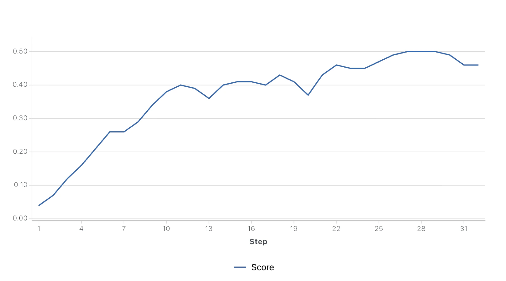
- You can leave most other hyperparameters as their defaults, though fine-tuning for 32 epochs (i.e., setting
Epochsto32) is recommended due to the complexity of the task. - Click “Create Job”.
- You can monitor the progress of your job in the Fine-Tuning tab. In this example, we trained for 32 epochs and got the following plot:
- Once the job status is
Completed, you can deploy your model. To deploy, click “Deploy” on the top right of your fine-tuning job’s page and then “Deploy LoRA Model”. Please note:- The Model under “Select base model*” should be the one from your Reinforcement Fine-Tuning job (this should be populated automatically)
- Speculative decoding is an advanced technique that can improve latency, but is not needed for this use-case
- Feel free to make the other selections (Performance, Scaling, and Metadata) as needed; enabling autoscaling is recommended to reduce costs
- Find this new model and click the Deploy button to create an API endpoint.
LLM_MODEL variable in the testing cell (step #13) to make sure it works as expected, along with your MCP server URL (i.e., LLM_MODEL = "accounts/<your-account-id>/models/<your-model-id>" and MCP_SERVER_URL = "<your-mcp-server-url>").
15. ⚖️ Evaluate Model Performance
Now for the moment of truth. We will systematically compare the performance of the original base model against our newly fine-tuned model, as well as a much larger base model, to quantify the improvement and general accuracy. We’ll run both models against every entry in our test dataset (final_rft_sql_test_data.jsonl). For each entry, we will:- Provide the same system and user prompt to both the base model and the fine-tuned model.
- Capture the SQL query generated by each.
- Execute each query against our live MCP server.
- Compare the query result to the ground_truth from our dataset.
- Keep a running score for each model.
Real World 🌍 This is a critical step in any MLOps loop. Evaluating a model on a consistent test set is the only way to prove that your efforts have resulted in a tangible improvement. In production, you’d also want to:
- Track latency and cost metrics
- Monitor for drift over time
- A/B test against your current solution
- Collect user feedback on query quality
16. ✨ Cleanup & Conclusion
Congratulations! You’ve successfully completed the entire Reinforcement Fine-Tuning loop. You started with just a database schema and ended with a highly specialized, performant, and data-aware AI model.Cleanup
Cloud resources and model deployments can incur costs, so it’s good practice to clean up any resources you no longer need.- Check your Deployments: Navigate to the Deployments tab in your Fireworks AI dashboard. Here you can monitor and manage all your deployed models.
- Delete Unneeded Models: Feel free to delete any deployments you no longer need. For example, you might have deployed the base or large-base models during the evaluation step to compare against your fine-tuned model. These can now be safely removed to save costs.
- Delete Cloud Run service and container image: Feel free to delete your MCP server Cloud Run service and container image to avoid stray storage costs.
Conclusions
The evaluation results from the previous step highlight the power of this approach.- Performance on par with massive models: Our fine-tuned 7B parameter model performs better than a much larger model like
qwen3-coder-480b-a35b-instructon this specific dataset. This is because it has been fine-tuned to understand the data schema via real query generation and execution. - Efficiency Gains: A 7B model is significantly faster and cheaper to run than a 480B one, offering production-grade performance at a fraction of the cost and latency.
- High-Level Capability on Complex Tasks: The queries in this dataset are relatively complex, which is reflected in the final accuracy score of around 57%. This is a strong result, demonstrating that for a specialized domain, a smaller model can be tuned to achieve a level of performance that exceeds larger models like
qwen3-coder-480b-a35b-instruct. Specifically, the final accuracy scores we measured for this dataset were:- Qwen2.5 7B (base): 23.91% accuracy (22/92 correct on the held-out test set)
- Qwen3 Coder 480B A35B Instruct (base): 34.78% accuracy (32/92 correct on the held-out test set)
- Qwen2.5 7B (RFT tuned): 56.52% accuracy (52/92 correct on the held-out test set)
Throughout this tutorial, we demonstrated a complete, end-to-end workflow for creating a fine-tuned text-to-SQL model. We began with the absolute minimum requirement, a database schema, and used a series of LLM-driven steps to generate a safe, synthetic data sandbox. From there, we generated a rich dataset of queries and answers, which we used to fine-tune a model using the Fireworks RFT platform. The final result is a small, efficient model that can accurately query data it has never seen, a task that was previously only possible with vastly larger and more expensive models. This pattern of schema → synthetic data → RFT is a secure, effective, and repeatable methodology for teaching language models to become expert users of your private data and custom APIs, without ever exposing the underlying sensitive information.
Appendix
Testing more open models on Fireworks
Testing proprietary models
Note that Claude Sonnet 4 and GPT-4o sometimes output SQL queries wrapped in markdown formatting like ```sql <query_here>```, so we added a helper function to clean the output before executing the SQL query in those cases.